Economic Regulation Authority Western Australia release Benchmark Reserve Capacity Prices for the 2028/29 capacity year, using six hour BESS as the Benchmark Technology.
Late last year we published a piece examining the importance of weather and stochastic variables to price outcomes. Since then, we have repeatedly been asked to explain how these stochastic variables behave, their influence on price outcomes, and the broader implications for the grid. We have been uplifting our own capabilities in modelling these stochastic factors. Most notably, we are increasingly conscious of the implications of there being a wide range of possible outcomes for reliability. Against this backdrop, in this article, we examine how outcomes differ when we alter weather and demand-supply (i.e., assumptions about adding or losing a major unit). We show that an analysis of median or average outcomes based on a single weather reference year, and a single set of demand assumptions is wholly inadequate for understanding variability, uncertainty and risk, and most importantly the reliability of the system. We want to stress test the system that is implied by a median set of conditions and see how it performs.
Moving from averages to distributions
The computational complexity of running market models means that it is costly in terms of time and computational resources to run many different simulations of the future. Average or ‘typical’ conditions are used as the basis for most long-term capacity expansion forecasts for this reason. Yet this is no longer enough. We cannot shoehorn a stochastic system into a deterministic model – we are misleading ourselves if we think that this will be adequate to guide us through the maze of complexity that awaits us in a high penetration renewable future.
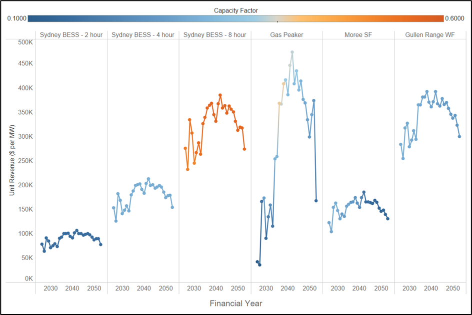
Figure 1 shows the average revenue per megawatt for a range of assets in NSW under a median weather reference year, and a single realisation of demand. For the purposes of this article, we have used Endgame’s Sunny-side up scenario as the basis for our forecasts. This scenario assumes a new build profile that is based on a median weather reference year, with a high (POE10) assumption about demand. The colour scale shows the capacity factor of each of the assets. We note the following:
Longer duration batteries make more money per MW of installed capacity.
Gas proves its value later in the horizon, as renewable penetration increases.
Wind makes solid returns because our modelling assumes constraints on the new build of this technology, limiting new entry from competing away profits.
Figure 1 – Revenue per MW for a single weather year for assets in NSW
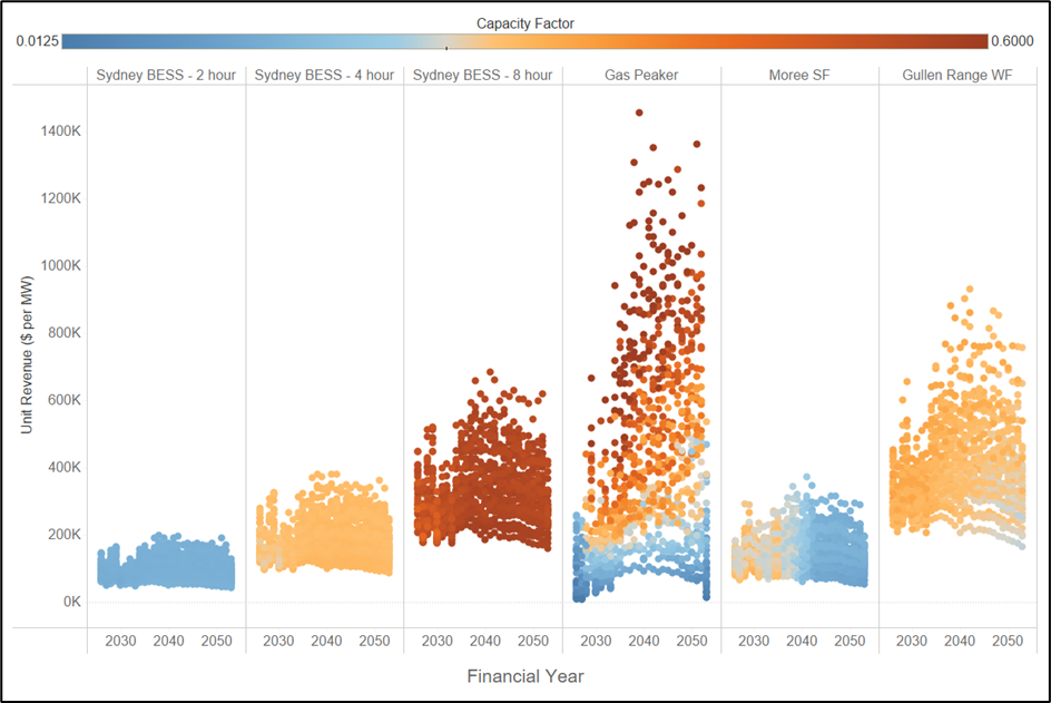
But how does this picture change when we consider many different reference years and allow for ups and downs in supply (eg, N-1 or N+1 relative to forecast). The result is shown in Figure 2. Each dot represents a single realisation of revenue per megawatt for a single year.
Figure 2 – Distribution of revenue per MW for 3 demand sensitivities, 13 weather years
We observe the following:
The upside for longer duration batteries is far greater than for shorter duration batteries.
The range of outcomes for wind is far greater than for solar.
The most striking outcome is that gas generation can earn super-normal profits in some years, and in other years it can fail to earn anything.
What does this mean for the gas supply system?
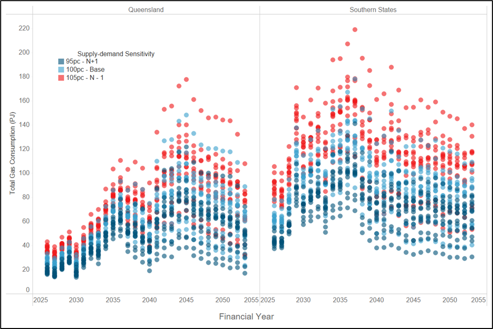
The differences between the outcomes in Figure 1 and Figure 2 completely changes how we should think about each of these assets, and the system as a whole. For example, consider the implications for gas consumption via gas-powered generation (GPG). Figure 3 shows the differences in total GPG consumption across each weather year and demand sensitivity. We can see differences in a given year of up to 120 PJ across the southern states.
Figure 3 – Distribution of GPG for 3 electricity demand sensitivities, 13 weather years
This gives rise to many questions, such as the following:
What does this mean for planning purposes?
What is the value of ‘insurance-style’ assets that can deliver gas in outlier years?
How resilient is our current system to these types of events?
How do we reward gas production and transportation and long duration pumped hydro facilities that may only be required with a low probability?
What does this mean for gas turbines that are contracting for gas supply?
Indeed, the consequences are too many to enumerate here. But the key point is that unless we understand the distribution of outcomes, we have no chance of planning for the future that awaits us.
Stress testing to understand reliability
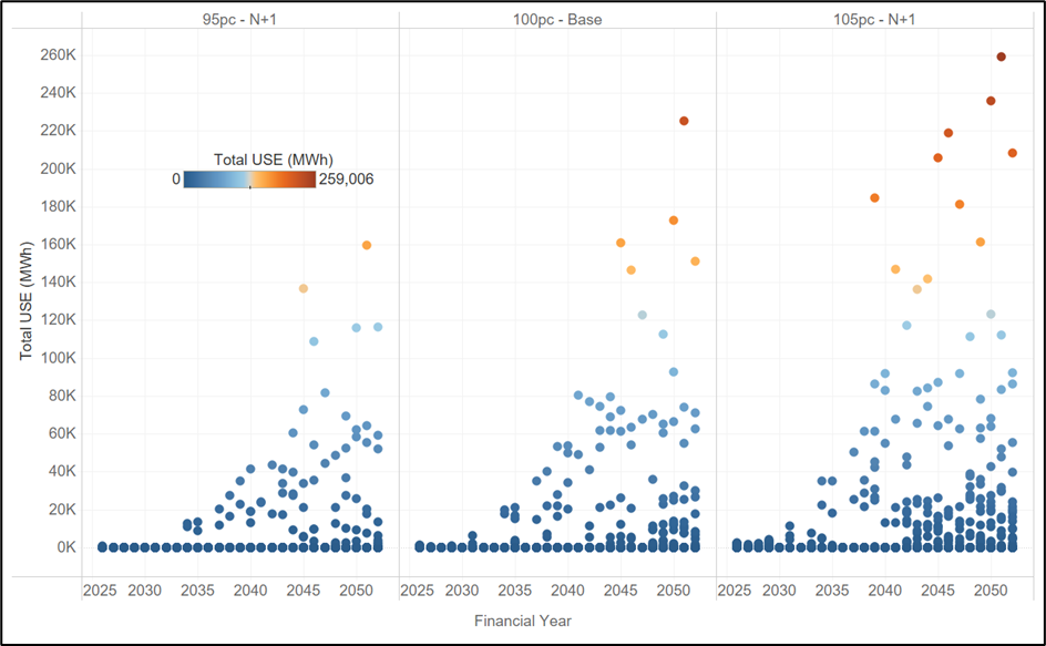
We have examined the consequences for gas, but what does this mean for system reliability? Our analysis shows that the variability of output for renewables has consequences for the reliance on gas. But what about unserved energy (USE) – ie, how often will weather and demand variability lead us to run short of generation, and how far are we at any point in time from shedding load?
Figure 4 below shows the consequences for unserved energy across 13 weather reference years and 3 demand-supply sensitivities. The result is that as renewable penetration increases over time, although the median conditions exhibit no USE, the distribution has long tails.
As the system becomes more stochastic, the importance of considering these extreme events only grows. By the 2040s we are in a situation where a shock to the system leads to outcomes that would not be considered reasonable by consumers (eg, 50-100 times the reliability standard in NSW). We note that these are driven by plausible and quantifiable variations in supply and demand, rather than ‘black swan’ events that may be examined by others in the sector.
Figure 4 – Projected USE in NSW for Sunny-side up scenario implied by distribution across 13 weather reference years and 3 demand-supply sensitivities.
This is not intended to be taken a criticism of renewables, but rather an observation that current modelling of single realisations of the future is inadequate to inform the needs of the system. We need a different approach. We make the following recommendations:
We need to start stress testing the system of the future, and understanding how variability in weather, demand, and gas supply influence reliability and resilience. In our opinion, the current ESOO is a solid starting point, but does not address the question of how we should go about filling the gaps that it identifies.
We need to think about how the assets that will provide resilience to these events will be rewarded in the market. Even with a very high market price cap, a generator that is only required under very extreme circumstances may never get built because of the challenges of obtaining financing for assets that are only used in 1 in 50 or 1 in 100 year events.
Finally, stress testing needs to consider all elements of the energy supply chain. From gas supply to hydrology and network availability. Models that can provide insights into these risks will help us build a system that exploits the many advantages of renewables, but recognises and addresses the blind spots of a high VRE system.
In conclusion, we need to understand that the nature of risk in this future system is fundamentally different to that which existed in our legacy system, and that our existing approaches may give highly misleading answers as to reliability and risk.
We have seen solar and batteries at the core of government schemes over the last year, and indeed further back in time. In addition, the Commonwealth has sought to make the most of solar resources by encouraging consumption during the middle of the day with its Solar Sharer Offer. And finally with the challenges facing the roll-out of wind, gas and pumped hydro projects, we are left in a world where many of our clients have said to us that solar is the only option for investment. Against this backdrop, we ask the question how hungry is our current market for solar, and what can we learn about the returns that solar will earn from the energy only market?
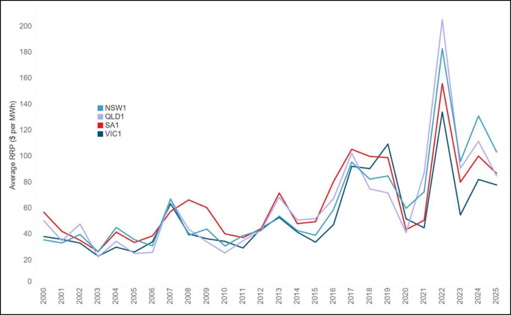
Average prices in 2025
As a starting point, we examine historical average prices for the mainland regions of the National Electricity Market (NEM). Figure 1 shows that 2025 prices were lower in all regions than 2024 prices but have risen from their levels in 2023. New South Wales experienced the highest average price of $103 per MWh, with Victoria the lowest at $77.9 per MWh.
Figure 1 – Average calendar year prices for mainland regions of the NEM, 2000-2025
Average prices for different periods of the day
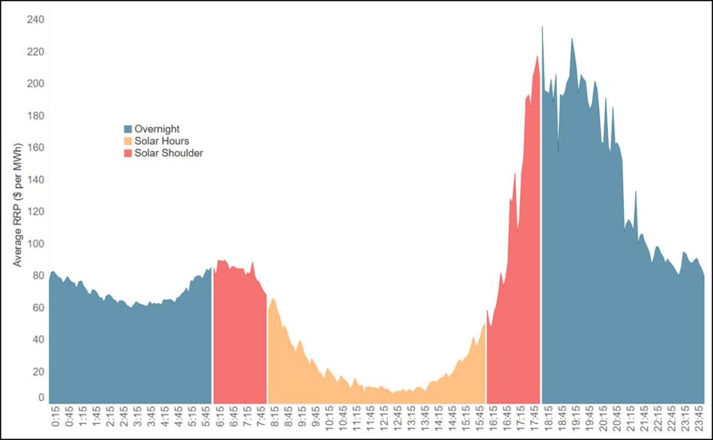
Average prices are a good starting point to understand the returns to solar, but the marked feature of prices over the last decade has been the deepening duck curve.
Figure 2 shows the average dispatch price by time of day for Victoria in 2025. We have coloured the different times of day according to solar output during these periods, namely:
Solar hours, which are 8 am to 4 pm.
Solar shoulder hours, which are 6 am to 8 am and 4 pm to 6 pm.
Overnight periods, from 6 pm to 6 am.
The belly of the duck (ie, the solar hours) is markedly lower than the shoulder and overnight periods, as has been seen for some time.
Figure 2 – 2025 average Victoria prices by time of day, coloured by solar definition
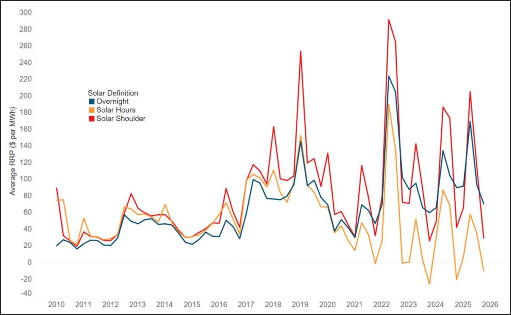
An immediate question is how prices for each of these time periods have changed over time with the increasing penetration of solar. Figure 3 shows the Victoria quarterly average price for each of the three categories: solar hours, solar shoulder, and overnight.
We note the following:
Over the period from 2010 to 2020, overnight and solar periods experienced very similar outcomes, but from 2021 onwards there has been a marked divergence between solar and overnight periods.
Prices for solar hours have collapsed in recent years and have now often become negative on average for entire quarters, namely Q4 2023, Q4 2024 and Q4 2025.
There is a clear quarterly pattern emerging with the highest prices in Q2 and Q3.
Figure 3 – Victoria quarterly average prices by solar category, 2010 to 2025
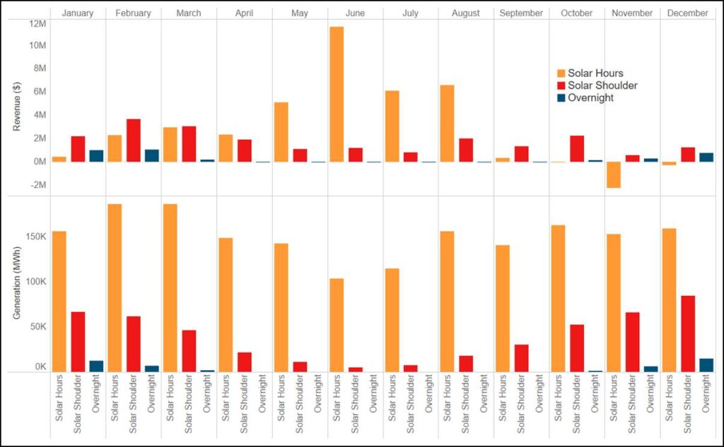
Bringing revenue into the equation
Average price is a very helpful indicator of the available pie for solar, but if we want to look more deeply at returns it is necessary to incorporate dispatch volumes, which vary greatly over the course of the year. With that in mind, Figure 4 shows the monthly revenue and generation by solar category for all solar farms in Victoria for 2025.
We note the following:
38 per cent of all revenue is earned in the solar shoulder, with the remainder coming from solar hours.
Counterintuitively, the vast majority (ie, 90 per cent) of revenue from solar periods is earned winter when output from solar is at its lowest. Indeed, revenue from solar periods was negative during Q4.
The relationship between generation and revenue is not straightforward – more generation does not necessarily lead to more revenue, because when we generate during the year matters.
Figure 4 – Revenue and generation across all solar units in Victoria by solar category
Looking to the future – solar earns the bulk of its revenue in winter
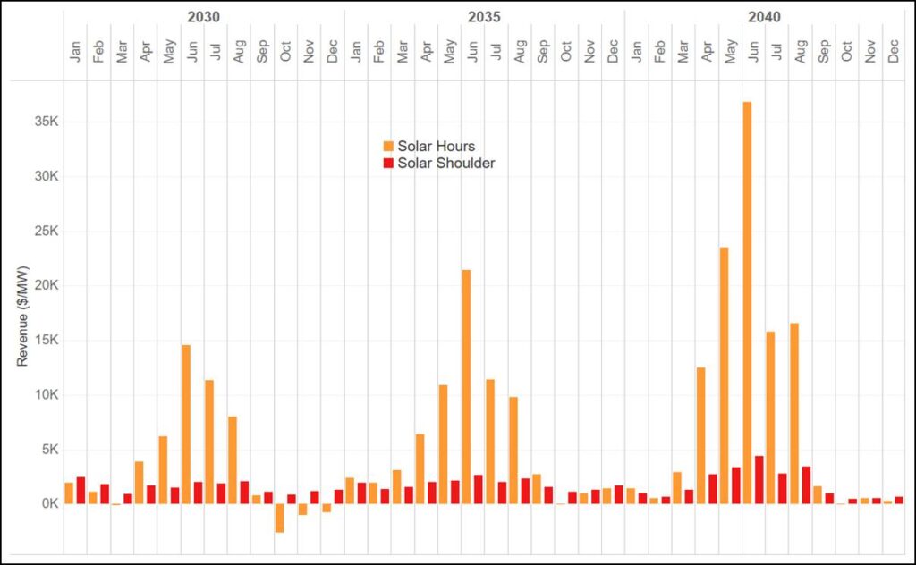
We can also project forward to see how the system will evolve using one of our house scenarios, ie, Endgame’s Sunny Side Up Scenario. Figure 5 shows average Victoria revenue per MW for three financial years by month and solar category for this case. We project that the pattern of the increasing significance of winter continues – indeed, by 2039-40 our modelling shows that solar will earn virtually nothing from September to March save for the small amount of output during the solar shoulders. In addition, the relative importance of the shoulder decreases from around 30 per cent of revenue to 16.5 per cent by FY2040.
Figure 5 – Projected Victoria solar revenue per MW; FY2030, FY2035, FY2040
What does this mean?
Solar revenues in summer have collapsed. Solar must now justify itself through contribution to the system during winter, particularly when the system is becalmed, ie, when wind output is low. Even with the large amounts of batteries that are projected to enter the system, this outcome does not change. The success of solar, and particularly rooftop solar, has led to a world where the system will be awash with energy in summer and so the marginal value of the technology is greatest when its output is relatively low.
We conclude with the following observations:
Solar earns most of its money when it is operating at a relatively low proportion of nameplate capacity. It follows that any curtailment which occurs during summer may be largely irrelevant to the overall revenue of a site.
Financiers need to be comfortable that they are buying an asset that makes most of its money when it is generating well beneath its capacity. Our own modelling shows that large proportions of solar revenue may come from periods where it is generating at less than 30 per cent of nameplate.
The massively seasonal nature of solar revenue makes a strong case for seasonal storage of any form of energy. Technologies that can move megawatt-hours between seasons will be extremely valuable in this context.
Given the large amount of variability in the occurrence and frequency of wind droughts from one year to the next, it follows that solar spot revenue will be incredible volatile. This is borne out by our own analysis of outcomes for different weather reference years. Batteries cannot mitigate this risk – deeper forms of energy storage and gas are required to hedge load.